
35 KiB
| title | author | date | isbn | publisher | category | chapter | pages |
|---|---|---|---|---|---|---|---|
| Michael Abrash's Graphics Programming Black Book, Special Edition | Michael Abrash | 1997-07-01 | 1576101746 | The Coriolis Group | Web and Software Development: Game Development,Web and Software Development: Graphics and Multimedia Development | 59 | 1095-1114 |
Chapter 59 -- The Idea of BSP Trees
What BSP Trees Are and How to Walk Them
The answer is: Wendy Tucker.
The question that goes with that answer isn't particularly interesting to anyone but me—but the manner in which I came up with the answer is.
I spent many of my childhood summers at Camp Chingacook, on Lake George in New York. It was a great place to have fun and do some growing up, with swimming and sailing and hiking and lots more.
When I was 14, Camp Chingacook had a mixer with a nearby girls' camp. As best I can recall, I had never had any interest in girls before, but after the older kids had paired up, I noticed a pretty girl looking at me and, with considerable trepidation, I crossed the room to talk to her. To my amazement, we hit it off terrifically. We talked non-stop for the rest of the evening, and I walked back to my cabin floating on air. I had taken a first, tentative step into adulthood, and my world would never be quite the same.
That was the only time I ever saw her, although I would occasionally remember that warm glow and call up an image of her smiling face. That happened less frequently as the years passed and I had real girlfriends, and by the time I got married, that particular memory was stashed in some back storeroom of my mind. I didn't think of her again for more than a decade.
A few days ago, for some reason, that mixer popped into my mind as I was trying to fall asleep. And I wondered, for the first time in 20 years, what that girl's name was. The name was there in my mind, somewhere; I could feel the shape of it, in that same back storeroom, if only I could figure out how to retrieve it.
I poked and worried at that memory, trying to get it to come to the surface. I concentrated on it as hard as I could, and even started going through the alphabet one letter at a time, trying to remember if her name started with each letter. After 15 minutes, I was wide awake and totally frustrated. I was also farther than ever from answering the question; all the focusing on the memory was beginning to blur the original imprint.
At this point, I consciously relaxed and made myself think about something completely different. Every time my mind returned to the mystery girl, I gently shifted it to something else. After a while, I began to drift off to sleep, and as I did a connection was made, and a name popped, unbidden, into my mind.
Wendy Tucker.
There are many problems that are amenable to the straight-ahead, purely conscious sort of approach that I first tried to use to retrieve Wendy's name. Writing code (once it's designed) is often like that, as are some sorts of debugging, technical writing, and balancing your checkbook. I personally find these left-brain activities to be very appealing because they're finite and controllable; when I start one, I know I'll be able to deal with whatever comes up and make good progress, just by plowing along. Inspiration and intuitive leaps are sometimes useful, but not required.
The problem is, though, that neither you nor I will ever do anything great without inspiration and intuitive leaps, and especially not without stepping away from what's known and venturing into territories beyond. The way to do that is not by trying harder but, paradoxically, by trying less hard, stepping back, and giving your right brain room to work, then listening for and nurturing whatever comes of that. On a small scale, that's how I remembered Wendy's name, and on a larger scale, that's how programmers come up with products that are more than me-too, checklist-oriented software.
Which, for a couple of reasons, brings us neatly to this chapter's topic, Binary Space Partitioning (BSP) trees. First, games are probably the sort of software in which the right-brain element is most important—blockbuster games are almost always breakthroughs in one way or another—and some very successful games use BSP trees, most notably id Software's megahit DOOM. Second, BSP trees aren't intuitively easy to grasp, and considerable ingenuity and inventiveness is required to get the most from them.
Before we begin, I'd like to thank John Carmack, the technical wizard behind DOOM, for generously sharing his knowledge of BSP trees with me.
BSP Trees
A BSP tree is, at heart, nothing more than a tree that subdivides space in order to isolate features of interest. Each node of a BSP tree splits an area or a volume (in 2-D or 3-D, respectively) into two parts along a line or a plane; thus the name "Binary Space Partitioning." The subdivision is hierarchical; the root node splits the world into two subspaces, then each of the root's two children splits one of those two subspaces into two more parts. This continues with each subspace being further subdivided, until each component of interest (each line segment or polygon, for example) has been assigned its own unique subspace. This is, admittedly, a pretty abstract description, but the workings of BSP trees will become clearer shortly; it may help to glance ahead to this chapter's figures.
Building a tree that subdivides space doesn't sound particularly profound, but there's a lot that can be done with such a structure. BSP trees can be used to represent shapes, and operating on those shapes is a simple matter of combining trees as needed; this makes BSP trees a powerful way to implement Constructive Solid Geometry (CSG). BSP trees can also be used for hit testing, line-of-sight determination, and collision detection.
Visibility Determination
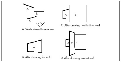
For the time being, I'm going to discuss only one of the many uses of BSP trees: The ability of a BSP tree to allow you to traverse a set of line segments or polygons in back-to-front or front-to-back order as seen from any arbitrary viewpoint. This sort of traversal can be very helpful in determining which parts of each line segment or polygon are visible and which are occluded from the current viewpoint in a 3-D scene. Thus, a BSP tree makes possible an efficient implementation of the painter's algorithm, whereby polygons are drawn in back-to-front order, with closer polygons overwriting more distant ones that overlap, as shown in Figure 59.1. (The line segments in Figure 1(a) and in other figures in this chapter, represent vertical walls, viewed from directly above.) Alternatively, visibility determination can be performed by front-to-back traversal working in conjunction with some method for remembering which pixels have already been drawn. The latter approach is more complex, but has the potential benefit of allowing you to early-out from traversal of the scene database when all the pixels on the screen have been drawn.
Back-to-front or front-to-back traversal in itself wouldn't be so impressive—there are many ways to do that—were it not for one additional detail: The traversal can always be performed in linear time, as we'll see later on. For instance, you can traverse, a polygon list back-to-front from any viewpoint simply by walking through the corresponding BSP tree once, visiting each node one and only one time, and performing only one relatively inexpensive test at each node.
It's hard to get cheaper sorting than linear time, and BSP-based rendering stacks up well against alternatives such as z-buffering, octrees, z-scan sorting, and polygon sorting. Better yet, a scene database represented as a BSP tree can be clipped to the view pyramid very efficiently; huge chunks of a BSP tree can be lopped off when clipping to the view pyramid, because if the entire area or volume of a node lies entirely outside the view volume, then all nodes and leaves that are children of that node must likewise be outside the view volume, for reasons that will become clear as we delve into the workings of BSP trees.
Limitations of BSP Trees
Powerful as they are, BSP trees aren't perfect. By far the greatest limitation of BSP trees is that they're time-consuming to build, enough so that, for all practical purposes, BSP trees must be precalculated, and cannot be built dynamically at runtime. In fact, a BSP-tree compiler that attempts to perform some optimization (limiting the number of surfaces that need to be split, for example) can easily take minutes or even hours to process large world databases.
A fixed world database is fine for walkthrough or flythrough applications (where the viewpoint moves through a static scene), but not much use for games or virtual reality, where objects constantly move relative to one another. Consequently, various workarounds have been developed to allow moving objects to appear in BSP tree-based scenes. DOOM, for example, uses 2-D sprites mixed into BSP-based 3-D scenes; note, though, that this approach requires maintaining z information so that sprites can be drawn and occluded properly. Alternatively, movable objects could be represented as separate BSP trees and merged anew into the world BSP tree with each move. Dynamic merging may or may not be fast enough, depending on the scene, but merging BSP trees tends to be quicker than building them, because the BSP trees being merged are already spatially sorted.
Another possibility would be to generate a per-pixel z-buffer for each frame as it's rendered, to allow dynamically changing objects to be drawn into the BSP-based world. In this scheme, the BSP tree would allow fast traversal and clipping of the complex, static world, and the z-buffer would handle the relatively localized visibility determination involving moving objects. The drawback of this is the need for a memory-hungry z-buffer; a typical 640x480 z-buffer requires a fairly appalling 600K, with equally appalling cache-miss implications for performance.
Yet another possibility would be to build the world so that each dynamic object falls entirely within a single subspace of the static BSP tree, rather than straddling splitting lines or planes. In this case, dynamic objects can be treated as points, which are then just sorted into the BSP tree on the fly as they move.
The only other drawbacks of BSP trees that I know of are the memory required to store the tree, which amounts to a few pointers per node, and the relative complexity of debugging BSP-tree compilation and usage; debugging a large data set being processed by recursive code (which BSP code tends to be) can be quite a challenge. Tools like the BSP compiler I'll present in the next chapter, which visually depicts the process of spatial subdivision as a BSP tree is constructed, help a great deal with BSP debugging.
Building a BSP Tree
Now that we know a good bit about what a BSP tree is, how it helps in visible surface determination, and what its strengths and weaknesses are, let's take a look at how a BSP tree actually works to provide front-to-back or back-to-front ordering. This chapter's discussion will be at a conceptual level, with plenty of figures; in the next chapter we'll get into mechanisms and implementation details.
I'm going to discuss only 2-D BSP trees from here on out, because they're much easier to draw and to grasp than their 3-D counterparts. Don't worry, though; the principles of 2-D BSP trees using line segments generalize directly to 3-D BSP trees using polygons. Also, 2-D BSP trees are quite powerful in their own right, as evidenced by DOOM, which is built around 2-D BSP trees.
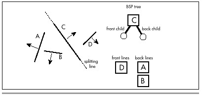
First, let's construct a simple BSP tree. Figure 59.2 shows a set of four lines that will constitute our sample world. I'll refer to these as walls, because that's one easily-visualized context in which a 2-D BSP tree would be useful in a game. Think of Figure 59.2 as depicting vertical walls viewed from directly above, so they're lines for the purpose of the BSP tree. Note that each wall has a front side, denoted by a normal (perpendicular) vector, and a back side. To make a BSP tree for this sample set, we need to split the world in two, then each part into two again, and so on, until each wall resides in its own unique subspace. An obvious question, then, is how should we carve up the world of Figure 59.2?

There are infinitely valid ways to carve up Figure 59.2, but the simplest is just to carve along the lines of the walls themselves, with each node containing one wall. This is not necessarily optimal, in the sense of producing the smallest tree, but it has the virtue of generating the splitting lines without expensive analysis. It also saves on data storage, because the data for the walls can do double duty in describing the splitting lines as well. (Putting one wall on each splitting line doesn't actually create a unique subspace for each wall, but it does create a unique subspace boundary for each wall; as we'll see, that spatial organization provides for the same unambiguous visibility ordering as a unique subspace would.)
Creating a BSP tree is a recursive process, so we'll perform the first split and go from there. Figure 59.3 shows the world carved along the line of wall C into two parts: walls that are in front of wall C, and walls that are behind. (Any of the walls would have been an equally valid choice for the initial split; we'll return to the issue of choosing splitting walls in the next chapter.) This splitting into front and back is the essential dualism of BSP trees.
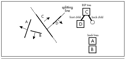
Next, in Figure 59.4, the front subspace of wall C is split by wall D. This is the only wall in that subspace, so we're done with wall C's front subspace.
Figure 59.5 shows the back subspace of wall C being split by wall B. There's a difference here, though: Wall A straddles the splitting line generated from wall B. Does wall A belong in the front or back subspace of wall B?
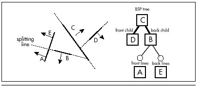
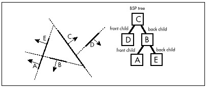
Both, actually. Wall A gets split into two pieces, which I'll call wall A and wall E; each piece is assigned to the appropriate subspace and treated as a separate wall. As shown in Figure 59.6, each of the split pieces then has a subspace to itself, and each becomes a leaf of the tree. The BSP tree is now complete.
Visibility Ordering
Now that we've successfully built a BSP tree, you might justifiably be a little puzzled as to how any of this helps with visibility ordering. The answer is that each BSP node can definitively determine which of its child trees is nearer and which is farther from any and all viewpoints; applied throughout the tree, this principle makes it possible to establish visibility ordering for all the line segments or planes in a BSP tree, no matter what the viewing angle.
Consider the world of Figure 59.2 viewed from an arbitrary angle, as shown in Figure 59.7. The viewpoint is in front of wall C; this tells us that all walls belonging to the front tree that descends from wall C are nearer along every ray from the viewpoint than wall C is (that is, they can't be occluded by wall C). All the walls in wall C's back tree are likewise farther away than wall C along any ray. Thus, for this viewpoint, we know for sure that if we're using the painter's algorithm, we want to draw all the walls in the back tree first, then wall C, and then the walls in the front tree. If the viewpoint had been on the back side of wall C, this order would have been reversed.
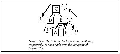
Of course, we need more ordering information than wall C alone can give us, but we get that by traversing the tree recursively, making the same far-near decision at each node. Figure 59.8 shows the painter's algorithm (back-to-front) traversal order of the tree for the viewpoint of Figure 59.7. At each node, we decide whether we're seeing the front or back side of that node's wall, then visit whichever of the wall's children is on the far side from the viewpoint, draw the wall, and then visit the node's nearer child, in that order. Visiting a child is recursive, involving the same far-near visiting order.

The key is that each BSP splitting line separates all the walls in the current subspace into two groups relative to the viewpoint, and every single member of the farther group is guaranteed not to occlude every single member of the nearer. By applying this ordering recursively, the BSP tree can be traversed to provide back-to-front or front-to-back ordering, with each node being visited only once.
The type of tree walk used to produce front-to-back or back-to-front BSP traversal is known as an inorder walk. More on this very shortly; you're also likely to find a discussion of inorder walking in any good data structures book. The only special aspect of BSP walks is that a decision has to be made at each node about which way the node's wall is facing relative to the viewpoint, so we know which child tree is nearer and which is farther.
Listing 59.1 shows a function that draws a BSP tree back-to-front. The
decision whether a node's wall is facing forward, made by
WallFacingForward() in Listing 59.1, can, in general, be made by
generating a normal to the node's wall in screenspace
(perspective-corrected space as seen from the viewpoint) and checking
whether the z component of the normal is positive or negative, or by
checking the sign of the dot product of a viewspace (non-perspective
corrected space as seen from the viewpoint) normal and a ray from the
viewpoint to the wall. In 2-D, the decision can be made by enforcing the
convention that when a wall is viewed from the front, the start vertex
is leftmost; then a simple screenspace comparison of the x coordinates
of the left and right vertices indicates which way the wall is facing.
Listing 59.1 L59_1.C
void WalkBSPTree(NODE *pNode)
{
   if (WallFacingForward(pNode) {
      if (pNode->BackChild) {
         WalkBSPTree(pNode->BackChild);
      }
      Draw(pNode);
      if (pNode->FrontChild) {
         WalkBSPTree(pNode->FrontChild);
      }
   } else {
      if (pNode->FrontChild) {
         WalkBSPTree(pNode->FrontChild);
      }
      Draw(pNode);
      if (pNode->BackChild) {
         WalkBSPTree(pNode->BackChild);
      }
   }
}
Be aware that BSP trees can often be made smaller and more efficient by detecting collinear surfaces (like aligned wall segments) and generating only one BSP node for each collinear set, with the collinear surfaces stored in, say, a linked list attached to that node. Collinear surfaces partition space identically and can't occlude one another, so it suffices to generate one splitting node for each collinear set.
Inorder Walks of BSP Trees
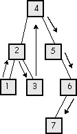
It was implementing BSP trees that got me to thinking about inorder tree traversal. In inorder traversal, the left subtree of each node gets visited first, then the node, and then the right subtree. You apply this sequence recursively to each node and its children until the entire tree has been visited, as shown in Figure 59.9. Walking a BSP tree is basically an inorder tree walk; the only difference is that with a BSP tree a decision is made before each descent as to which subtree to visit first, rather than simply visiting whatever's pointed to by the left-subtree pointer. Conceptually, however, an inorder walk is what's used to traverse a BSP tree; from now on I'll discuss normal inorder walking, with the understanding that the same principles apply to BSP trees.
As I've said again and again in my printed works over the years, you have to dig deep below the surface to really understand something if you want to get it right, and inorder walking turns out to be an excellent example of this. In fact, it's such a good example that I routinely use it as an interview question for programmer candidates, and, to my astonishment, not one interviewee has done a good job with this one yet. I ask the question in two stages, and I get remarkably consistent results.
First, I ask for an implementation of a function WalkTree() that
visits each node in a passed-in tree in inorder sequence. Each candidate
unhesitatingly writes something like the perfectly good code in Listings
59.2 and 59.3 shown next.
Listing 59.2 L59_2.C
// Function to inorder walk a tree, using code recursion.
// Tested with 32-bit Visual C++ 1.10.
#include <stdlib.h>
#include "tree.h"
extern void Visit(NODE *pNode);
void WalkTree(NODE *pNode)
{
   // Make sure the tree isn't empty
   if (pNode != NULL)
   {
      // Traverse the left subtree, if there is one
      if (pNode->pLeftChild != NULL)
      {
         WalkTree(pNode->pLeftChild);
      }
      // Visit this node
      Visit(pNode);
      // Traverse the right subtree, if there is one
      if (pNode->pRightChild != NULL)
      {
         WalkTree(pNode->pRightChild);
      }
   }
}
Listing 59.3 L59_3.H
// Header file TREE.H for tree-walking code.
typedef struct _NODE {
  struct _NODE *pLeftChild;
  struct _NODE *pRightChild;
} NODE;
Then I ask if they have any idea how to make the code faster; some don't, but most point out that function calls are pretty expensive. Either way, I then ask them to rewrite the function without code recursion.
And then I sit back and squirm for a minimum of 15 minutes.
I have never had anyone write a functional data-recursion inorder walk function in less time than that, and several people have simply never gotten the code to work at all. Even the best of them have fumbled their way through the code, sticking in a push here or a pop there, then working through sample scenarios in their head to see what's broken, programming by trial and error until the errors seem to be gone. No one is ever sure they have it right; instead, when they can't find any more bugs, they look at me hopefully to see if it's thumbs-up or thumbs-down.
And yet, a data-recursive inorder walk implementation has exactly the same flowchart and exactly the same functionality as the code-recursive version they've already written. They already have a fully functional model to follow, with all the problems solved, but they can't make the connection between that model and the code they're trying to implement. Why is this?
Know It Cold
The problem is that these people don't understand inorder walking
through and through. They understand the concepts of visiting left and
right subtrees, and they have a general picture of how traversal moves
about the tree, but they do not understand exactly what the
code-recursive version does. If they really comprehended everything that
happens in each iteration of WalkTree()—how each call saves the
state, and what that implies for the order in which operations are
performed—they would simply and without fuss implement code like that in
Listing 59.4, working with the code-recursive version as a model.
Listing 59.4 L59_4.C
// Function to inorder walk a tree, using data recursion.
// No stack overflow testing is performed.
// Tested with 32-bit Visual C++ 1.10.
#include <stdlib.h>
#include "tree.h"
#define MAX_PUSHED_NODES   100
extern void Visit(NODE *pNode);
void WalkTree(NODE *pNode)
{
   NODE *NodeStack[MAX_PUSHED_NODES];
   NODE **pNodeStack;
   // Make sure the tree isn't empty
   if (pNode != NULL)
   {
      NodeStack[0] = NULL;  // push "stack empty" value
      pNodeStack = NodeStack + 1;
      for (;;)
      {
         // If the current node has a left child, push
         // the current node and descend to the left
         // child to start traversing the left subtree.
         // Keep doing this until we come to a node
         // with no left child; that's the next node to
         // visit in inorder sequence
         while (pNode->pLeftChild != NULL)
         {
            *pNodeStack++ = pNode;
            pNode = pNode->pLeftChild;
         }
         // We're at a node that has no left child, so
         // visit the node, then visit the right
         // subtree if there is one, or the last-
         // pushed node otherwise; repeat for each
         // popped node until one with a right
         // subtree is found or we run out of pushed
         // nodes (note that the left subtrees of
         // pushed nodes have already been visited, so
         // they're equivalent at this point to nodes
         // with no left children)
         for (;;)
         {
            Visit(pNode);
            // If the node has a right child, make
            // the child the current node and start
            // traversing that subtree; otherwise, pop
            // back up the tree, visiting nodes we
            // passed on the way down, until we find a
            // node with a right subtree to traverse
            // or run out of pushed nodes and are done
            if (pNode->pRightChild != NULL)
            {
               // Current node has a right child;
               // traverse the right subtree
               pNode = pNode->pRightChild;
               break;
            }
            // Pop the next node from the stack so
            // we can visit it and see if it has a
            // right subtree to be traversed
            if ((pNode = *—pNodeStack) == NULL)
            {
               // Stack is empty and the current node
               // has no right child; we're done
               return;
            }
         }
      }
   }
}
Take a few minutes to look over Listing 59.4 and relate it to Listing 59.2. The structure is different, but upon examination it becomes clear that both listings reflect the same underlying model: For each node, visit the left subtree, visit the node, visit the right subtree. And although Listing 59.4 is longer, that's mostly because I commented it heavily to make sure its workings are understood; there are only 13 lines that actually do anything in Listing 59.4.
Let's look at it another way. All the code in Listing 59.2 does is say:
"Here I am at a node. First I'll visit the left subtree if there is one,
then I'll visit this node, then I'll visit the right subtree if there is
one. While I'm visiting the left subtree, I'll just push a marker on a
stack that tells me to come back here when the left subtree is done. If,
after visiting a node, there are no right children to visit and nothing
left on the stack, I'm finished. The code does this at each node—and
that's all it does. That's all Listing 59.4 does, too, but people tend
to get tangled up in pushes and pops and while loops when they use
data recursion. When the implementation model changes to one with which
they are unfamiliar, they abandon the perfectly good model they used
before and try to rederive it in the new context by the seat of their
pants.
The alternative is to develop and apply a unifying model. There aren't really two types of right children; the rule is that all right children are visited after their parents are visited, period. The presence or absence of a left child is irrelevant. The possibility that a right child may be reached via different code paths depending on the presence of a left child does not affect the overall model. While this distinction may seem trivial it is in fact crucial, because if you have the model down cold, you can always tell if the implementation is correct by comparing it with the model.
Measure and Learn
How much difference does all this fuss make, anyway? Listing 59.5 is a
sample program that builds a tree, then calls WalkTree () to walk it
1,000 times, and times how long this takes. Using 32-bit Visual C++ 1.10
running on Windows NT, with default optimization selected, Listing 59.5
reports that Listing 59.4 is about 20 percent faster than Listing 59.2
on a 486/33, a reasonable return for a little code rearrangement,
especially when you consider that the speedup is diluted by calling the
Visit() function and by the cache miss that happens on virtually
every node access. (Listing 59.5 builds a rather unique tree, one in
which every node has exactly two children. Different sorts of trees can
and do produce different performance results. Always know what you're
measuring!)
Listing 59.5 L59_5.C
// Sample program to exercise and time the performance of
// implementations of WalkTree().
// Tested with 32-bit Visual C++ 1.10 under Windows NT.
#include <stdio.h>
#include <conio.h>
#include <stdlib.h>
#include <time.h>
#include "tree.h"
long VisitCount = 0;
void main(void);
void BuildTree(NODE *pNode, int RemainingDepth);
extern void WalkTree(NODE *pRootNode);
void main()
{
   NODE RootNode;
   int i;
   long StartTime;
   // Build a sample tree
   BuildTree(&RootNode, 14);
   // Walk the tree 1000 times and see how long it takes
   StartTime = time(NULL);
   for (i=0; i<1000; i++)
   {
      WalkTree(&RootNode);
   }
   printf("Seconds elapsed: %ld\n",
           time(NULL) - StartTime);
   getch();
}
//
// Function to add right and left subtrees of the
// specified depth off the passed-in node.
//
void BuildTree(NODE *pNode, int RemainingDepth)
{
   if (RemainingDepth == 0)
   {
      pNode->pLeftChild = NULL;
      pNode->pRightChild = NULL;
   }
   else
   {
      pNode->pLeftChild = malloc(sizeof(NODE));
      if (pNode->pLeftChild == NULL)
      {
         printf("Out of memory\n");
         exit(1);
      }
      pNode->pRightChild = malloc(sizeof(NODE));
      if (pNode->pRightChild == NULL)
      {
         printf("Out of memory\n");
         exit(1);
      }
      BuildTree(pNode->pLeftChild, RemainingDepth - 1);
      BuildTree(pNode->pRightChild, RemainingDepth - 1);
   }
}
//
// Node-visiting function so WalkTree() has something to
// call.
//
void Visit(NODE *pNode)
{
   VisitCount++;
}
Things change when maximum optimization is selected, however: The
performance of the two implementations becomes virtually identical! How
can this be? Part of the answer is that the compiler does an amazingly
good job with Listing 59.2. Most impressively, when compiling Listing
59.2, the compiler actually converts all right-subtree descents from
code recursion to data recursion, by simply jumping back to the
left-subtree handling code instead of recursively calling
WalkTree(). This means that half the time Listing 59.4 has no
advantage over Listing 59.2; in fact, it's at a disadvantage because the
code that the compiler generates for handling right-subtree descent in
Listing 59.4 is somewhat inefficient, but the right-subtree code in
Listing 59.2 is a marvel of code generation, at just 3 instructions.
What's more, although left-subtree traversal is more efficient with data
recursion than with code recursion, the advantage is only four
instructions, because only one parameter is passed and because the
compiler doesn't bother setting up an EBP-based stack frame, instead it
uses ESP to address the stack. (And, in fact, this cost could be reduced
still further by eliminating the check for a NULL pNode at all but
the top level.) There are other interesting aspects to what the compiler
does with Listings 59.2 and 59.4 but that's enough to give you the idea.
It's worth noting that the compiler might not do as well with code
recursion in a more complex function, and that a good assembly language
implementation could probably speed up Listing 59.4 enough to make it
measurably faster than Listing 59.2, but not even close to being
enough faster to be worth the effort.
The moral of this story (apart from it being a good idea to enable compiler optimization) is:
-
Understand what you're doing, through and through.
-
Build a complete and consistent model in your head.
-
Design from the principles that the model provides.
-
Implement the design.
-
Measure to learn what you've wrought.
-
Go back to step 1 and apply what you've just learned.
With each iteration you'll dig deeper, learn more, and improve your ability to know where and how to focus your design and programming efforts. For example, with the C compilers I used five to 10 years ago, back when I learned about the relative strengths and weaknesses of code and data recursion, and with the processors then in use, Listing 59.4 would have blown away Listing 59.2. While doing this chapter, I've learned that given current processors and compiler technology, data recursion isn't going to get me any big wins; and yes, that was news to me. That's good; this information saves me from wasted effort in the future and tells me what to concentrate on when I use recursion.
Assume nothing, keep digging deeper, and never stop learning and growing. The world won't hold still for you, but fortunately you can run fast enough to keep up if you just keep at it.
Depths within depths indeed!
Surfing Amidst the Trees
In the next chapter, we'll build a BSP-tree compiler, and after that, we'll put together a rendering system built around the BSP trees the compiler generates. If the subject of BSP trees really grabs your fancy (as it should if you care at all about performance graphics) there is at this writing (February 1996) a World Wide Web page on BSP trees that you must investigate at http://www.qualia.com/bspfaq/. It's set up in the familiar Internet Frequently Asked Questions (FAQ) style, and is very good stuff.
Related Reading
Foley, J., A. van Dam, S. Feiner, and J. Hughes, Computer Graphics: Principles and Practice (Second Edition), Addison Wesley, 1990, pp. 555-557, 675-680.
Fuchs, H., Z. Kedem, and B. Naylor, "On Visible Surface Generation by A Priori Tree Structures," Computer Graphics Vol. 17(3), June 1980, pp. 124-133.
Gordon, D., and S. Chen, "Front-to-Back Display of BSP Trees," IEEE Computer Graphics and Applications, September 1991, pp. 79-85.
Naylor, B., "Binary Space Partitioning Trees as an Alternative Representation of Polytopes," Computer Aided Design, Vol. 22(4), May 1990, pp. 250-253.